demuxSNP: supervised demultiplexing using cell hashing and SNPs
Michael Lynch
University of LimerickAedin Culhane
University of LimerickSource:
vignettes/c-demuxSNP-package-demo.Rmd
c-demuxSNP-package-demo.Rmd
library(demuxSNP)
library(ComplexHeatmap)
library(viridisLite)
library(Seurat)
library(ggpubr)
library(dittoSeq)
library(utils)
library(EnsDb.Hsapiens.v86)
library(kableExtra)Introduction
To refresh, demultiplexing allows reduction of sequencing costs by sequencing cells from multiple biological samples on the same lane, as well as allowing identifying of the increased proportion of doublets associated with greater cells loaded. Poor demultiplexing performance results in waste in valuable data, reduction in LFC used in DE or otherwise potentially misleading results.
Existing Methods
Limitations of existing methods:
Hashing algorithms can correctly call some but not all cells correctly and is highly dependent on the hashing quality
SNPs algorithms either: Genotype based methods incur additoinal cost (Demuxlet) Genotype-free methods struggle to identify rarer samples (due to lack of genotype information)
demuxSNP Motivation
With cell hashing, we can confidently demultiplex some but not all cells. Using these high confidence cells, we can learn the SNPs associated with each group. This SNP information can then be used to assign remaining cells (which we could not confidently call using cell hashing) to their most similar group based on their SNP profile.
Novel features:
Uses both cell hashing and SNP data. Current methods are limited to using one or the other.
Selects SNPs based on being located in a gene expressed in a large proportion of cells to reduce noise, computational cost and increase interpretability.
Impact:
- Users can visually confirm validity (or lack thereof) of existing demultiplexing results in a tangible manner.
- Users can recover otherwise high quality cells which could not be confidently assigned using other methods.
- Cells from groups which are present in lower proportions may be classified better than with unsupervised SNP approaches.
Note: the approach used here differs from most SNP methods in that it is supervised. We attain knowledge of which SNPs are associated with which patients from the high confidence cells then use this to train a classifier. It is similar to demuxlet in the sense that the classifier uses group specific SNP information, however our method does not require the expense of genotyping and so may be much more widely applicable.
Installation
##biocdevel

if (!require("BiocManager", quietly = TRUE))
    install.packages("BiocManager")

BiocManager::install("demuxSNP")

## or for development version:

devtools::install_github("michaelplynch/demuxSNP")
Quick Usage
For full list of arguments and explanation of each function, please refer to relevant documentation.
Workflow
#Data loading
data(multiplexed_scrnaseq_sce,
     commonvariants_1kgenomes_subset,
     vartrix_consensus_snps,
     package = "demuxSNP")

small_sce<-multiplexed_scrnaseq_sce[,1:100]
ensdb <- EnsDb.Hsapiens.v86::EnsDb.Hsapiens.v86

#Preprocessing
top_genes<-common_genes(small_sce)
vcf_sub<-subset_vcf(commonvariants_1kgenomes_subset, top_genes, ensdb)
small_sce<-high_conf_calls(small_sce)

#Use subsetted vcf with VarTrix in default 'consensus' mode to generate SNPs
#matrix

small_sce<-add_snps(small_sce,vartrix_consensus_snps[,1:100])

small_sce<-reassign(small_sce,k=5)

table(small_sce$knn)
#>
#>  Doublet Hashtag1 Hashtag3 Hashtag4 Hashtag5 Hashtag6
#>       24       11       16        7       10       32
Function Explanation
top_genes <- common_genes(sce): Returns the genes
which are expressed (expression > 0) in the highest proportion of
cells. These genes are used below to subset the .vcf file.
new_vcf <- subset_vcf(vcf = vcf, top_genes = top_genes, ensdb = ensdb):
Subsets a supplied .vcf to SNP locations within the genes supplied. The
ranges of the genes are extracted from the EnsDb object.
sce <- high_conf_calls(sce = sce, assay = "HTO"):
Takes a SingleCellExperiment object with HTO altExp, runs demuxmix
and returns a factor of assigned labels, a logical vector indicating
high confidence calls and a logical vector indicating which cells to
predict (all).
sce <- add_snps(sce = sce, mat = vartrix_consensus_snps, thresh = 0.8):
Adds the SNP data from VarTrix (default consensus mode) to the
SingleCellExperiment object as an altExp. Additionally, filters out SNPs
with no reads in less than ‘thresh’ proportion of cells.
sce <- reassign(sce,
    k = 10,
    d = 10,
    train_cells = sce$train,
    predict_cells = sce$predict
)
Reassigns cells based on SNP profiles of high confidence cells. Singlet training data is based on high confidence singlet assignment. Doublets are simulated by systematically sampling and combining the SNP profiles of n cells pairs from each grouping combination. Cells to be used for training data are specified by “train_cells” (logical). Cells to be used for prediction are specified by “predict_cells” (logical), this may also include the training data.
Exploratory Analysis
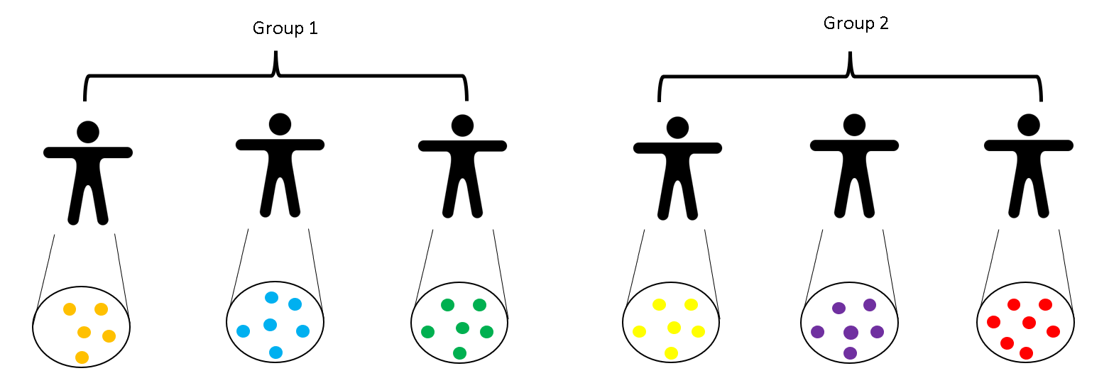
The sample dataset contains hashtag and SNP data from a sequencing run of six samples containing two grups to be compared:
knitr::include_graphics("./images/ccrcc-samples.png")
Multiplexed scRNASeq sample dataset
We load three data objects: a SingleCellExperiment object containing RNA and HTO counts, a .vcf file of class CollapsedVCF containing SNPs from 1000 Genomes common variants and a matrix containing SNP information for each cell (we will show you how to generate this SNPs matrix using VarTrix outside of R). We have already removed low quality cells (library size<1,000 and percentage of genes mapping to mitochondrial genes>10%).
class(multiplexed_scrnaseq_sce)
#> [1] "SingleCellExperiment"
#> attr(,"package")
#> [1] "SingleCellExperiment"
class(commonvariants_1kgenomes_subset)
#> [1] "CollapsedVCF"
#> attr(,"package")
#> [1] "VariantAnnotation"
class(vartrix_consensus_snps)
#> [1] "matrix" "array"
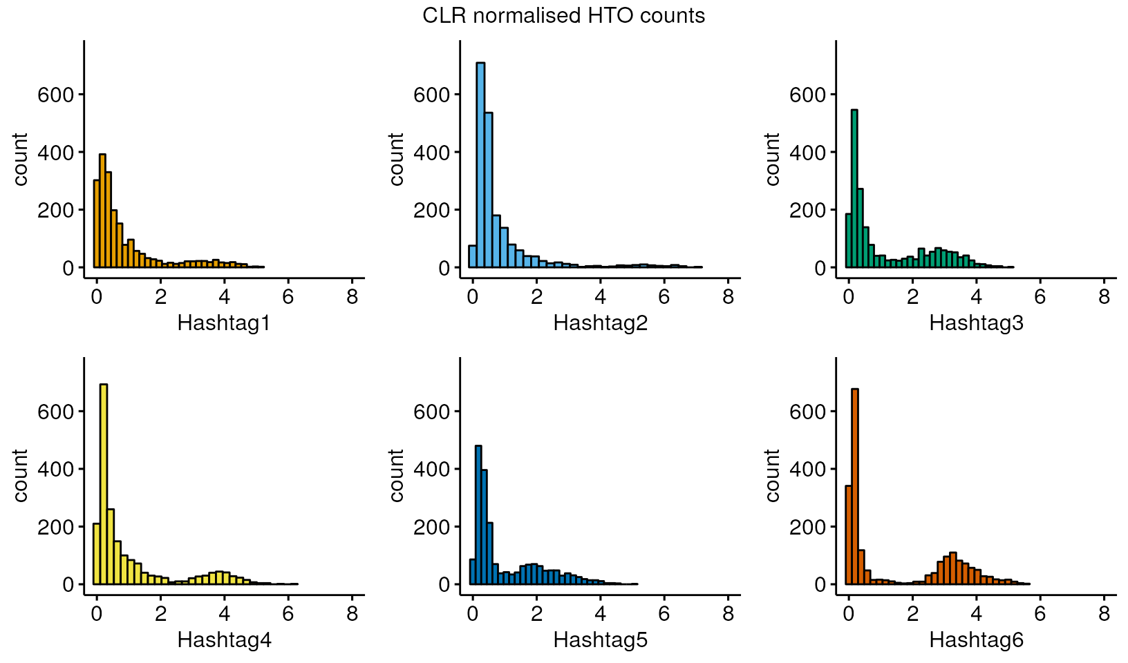
The HTO or LMO distribution is usually bimodal, with a signal (high counts) and background distribution (low counts) caused by non-specific binding. Ideally, these distributions would be clearly separated with no overlap, but in practice, this is not always the case. In our example data, we see that the signal and noise overlap to varying extents in each group.

We will begin by running Seurat’s HTODemux, a popular HTO demultiplexing algorithm on the data.
logcounts(multiplexed_scrnaseq_sce) <- counts(multiplexed_scrnaseq_sce)
seurat <- as.Seurat(multiplexed_scrnaseq_sce)
seurat <- HTODemux(seurat)
seurat <- MULTIseqDemux(seurat)
seurat$hash.ID <- factor(as.character(seurat$hash.ID))
seurat$MULTI_ID <- factor(as.character(seurat$MULTI_ID))

multiplexed_scrnaseq_sce$seurat <- seurat$hash.ID
multiplexed_scrnaseq_sce$multiseq<- seurat$MULTI_ID

t<-table(multiplexed_scrnaseq_sce$seurat)
u<-as.matrix(t)
kable(u) %>% kable_styling(bootstrap_options = "bordered")| Doublet | 633 |
| Hashtag1 | 121 |
| Hashtag2 | 29 |
| Hashtag3 | 264 |
| Hashtag4 | 158 |
| Hashtag5 | 177 |
| Hashtag6 | 383 |
| Negative | 235 |
Although HTO library size of the Negative group is low, the RNA library size is similar to that of other groups, indicating that they may be misclassified as ‘Negative’ due to their tagging quality rather than overall RNA quality.


library(CiteFuse)
multiplexed_scrnaseq_sce<-crossSampleDoublets(multiplexed_scrnaseq_sce)
#> number of iterations= 79
#> number of iterations= 60
#> number of iterations= 72
#> number of iterations= 80
#> number of iterations= 49
#> number of iterations= 73

kable(as.matrix(table(seurat$hash.ID,multiplexed_scrnaseq_sce$doubletClassify_between_label))) %>% kable_styling(bootstrap_options = "bordered")| 1 | 2 | 3 | 4 | 5 | 6 | doublet/multiplet | negative | |
|---|---|---|---|---|---|---|---|---|
| Doublet | 0 | 0 | 0 | 0 | 0 | 0 | 633 | 0 |
| Hashtag1 | 80 | 0 | 0 | 0 | 0 | 0 | 41 | 0 |
| Hashtag2 | 0 | 19 | 0 | 0 | 0 | 0 | 10 | 0 |
| Hashtag3 | 0 | 0 | 166 | 0 | 0 | 0 | 98 | 0 |
| Hashtag4 | 0 | 0 | 0 | 121 | 0 | 0 | 37 | 0 |
| Hashtag5 | 0 | 0 | 0 | 0 | 109 | 0 | 68 | 0 |
| Hashtag6 | 0 | 0 | 0 | 0 | 0 | 206 | 177 | 0 |
| Negative | 1 | 1 | 20 | 1 | 146 | 3 | 55 | 8 |
table(multiplexed_scrnaseq_sce$seurat,multiplexed_scrnaseq_sce$multiseq)
#>
#>            Doublet Hashtag1 Hashtag2 Hashtag3 Hashtag4 Hashtag5 Hashtag6
#>   Doublet      445       13        5       32       22       41       70
#>   Hashtag1       4       99        0        0        0        6        0
#>   Hashtag2       1        0       20        0        0        3        0
#>   Hashtag3       9        0        0      204        0        2        0
#>   Hashtag4       6        0        0        0      135        0        0
#>   Hashtag5       0        0        0        0        0      177        0
#>   Hashtag6      12        0        0        0        0        0      353
#>   Negative       0        0        0        0        0      129        0
#>
#>            Negative
#>   Doublet         5
#>   Hashtag1       12
#>   Hashtag2        5
#>   Hashtag3       49
#>   Hashtag4       17
#>   Hashtag5        0
#>   Hashtag6       18
#>   Negative      106

table(multiplexed_scrnaseq_sce$multiseq,multiplexed_scrnaseq_sce$doubletClassify_between_label)
#>
#>              1   2   3   4   5   6 doublet/multiplet negative
#>   Doublet    0   0   0   0   0   0               477        0
#>   Hashtag1  68   0   0   0   0   0                44        0
#>   Hashtag2   0  15   0   0   0   0                10        0
#>   Hashtag3   0   0 125   0   0   0               111        0
#>   Hashtag4   0   0   0 109   0   0                48        0
#>   Hashtag5   0   0   0   0 202   0               156        0
#>   Hashtag6   0   0   0   0   0 193               230        0
#>   Negative  13   5  61  13  53  16                43        8
For the remainder of this vignette we will outline our method of checking whether or not these cells have been called correctly and how to assign them to their appropriate group!
Preprocessing
Common variants files, for example from the 1000 Genomes Project, can contain over 7 million SNPs. To reduce computational cost and cell-type effects, we subset our SNPs list to those located within genes expressed across most cells in our data.
We first find the most commonly expressed genes in our RNA data.
top_genes <- common_genes(sce = multiplexed_scrnaseq_sce, n = 100)

top_genes[1:10]
#>  [1] "TPT1"   "RPL13"  "RPL28"  "TMSB4X" "RPS27"  "EEF1A1" "RPL41"  "B2M"
#>  [9] "RPLP1"  "RPL32"
We have a sample .vcf preloaded, but you can load your .vcf file in using ‘readVcf()’ from VariantAnnotation.
We will subset our .vcf file to SNPs seen in commonly expressed genes from our dataset. Notice that the genome for the vcf and EnsDb object must be compatible!
The returned vcf can be written to file and used with VarTrix later on.
ensdb <- EnsDb.Hsapiens.v86::EnsDb.Hsapiens.v86

genome(commonvariants_1kgenomes_subset)[1] == genome(ensdb)[1]
#>    1
#> TRUE

new_vcf <- subset_vcf(commonvariants_1kgenomes_subset, top_genes = top_genes, ensdb)
commonvariants_1kgenomes_subset
#> class: CollapsedVCF
#> dim: 2609 0
#> rowRanges(vcf):
#>   GRanges with 5 metadata columns: paramRangeID, REF, ALT, QUAL, FILTER
#> info(vcf):
#>   DataFrame with 1 column: AF
#> info(header(vcf)):
#>       Number Type  Description
#>    AF A      Float Estimated allele frequency in the range (0,1)
#> geno(vcf):
#>   List of length 0:
new_vcf
#> class: CollapsedVCF
#> dim: 2399 0
#> rowRanges(vcf):
#>   GRanges with 5 metadata columns: paramRangeID, REF, ALT, QUAL, FILTER
#> info(vcf):
#>   DataFrame with 1 column: AF
#> info(header(vcf)):
#>       Number Type  Description
#>    AF A      Float Estimated allele frequency in the range (0,1)
#> geno(vcf):
#>   List of length 0:
The subsetted .vcf can be written to disk using ‘writeVcf()’, again from VariantAnnotation package.
Next, we wish to identify cells which we can confidently call to a particular group. There are a number of ways this can be achieved, including probabilistic modelling of the HTO counts, manually setting non-conservative thresholds or using consensus calls. The user may wish to experiment with different approaches. Here we have used demuxmix, a probabilistic model which we have set with a high acceptance threshold to identify high confidence cell calls to use as training data (cells which we can confidently call as a particular singlet group).
multiplexed_scrnaseq_sce <- high_conf_calls(multiplexed_scrnaseq_sce)

table(multiplexed_scrnaseq_sce$train)
#>
#> FALSE  TRUE
#>   955  1045

table(multiplexed_scrnaseq_sce$predict)
#>
#> TRUE
#> 2000

table(multiplexed_scrnaseq_sce$labels)
#>
#>  Hashtag1  Hashtag2  Hashtag3  Hashtag4  Hashtag5  Hashtag6 multiplet  negative
#>        62        15       226       102       348       292       335        12
#> uncertain
#>       608
So, for this particular dataset, we can confidently call 1,045 cells as being from a particular singlet group. 608 cells cannot be called to a group with high confidence.
Variant Calling (VarTrix)
Variant calling is not done within the package. Instead, we refer the reader to VarTrix, where they can use the subsetted .vcf file along with their .bam, barcodes.tsv and reference genome to call SNPs in each cell.
A sample VarTrix command looks like the following:
./vartrix -v <path_to_input_vcf> -b <path_to_cellranger_bam> -f <path_to_fasta_file> -c <path_to_cell_barcodes_file> -o <path_for_output_matrix>Using the output matrix from Vartrix and the high confidence classifications from the HTO algorithm, we can reassign cells using k-nearest neighbours.
Cell Reassignment, Visualisation and Evaluation
To keep things tidy, we will add the SNP data to our SingleCellExperiment object as an altExp. We recode the SNP matrix as follows: 0=no read, 1=SNP present, -1=SNP absent. This function also filters out SNPs which are observed at a low frequency in the data, and the frequency threshold can be set manually.
dim(vartrix_consensus_snps)
#> [1] 2542 2000

multiplexed_scrnaseq_sce <- add_snps(multiplexed_scrnaseq_sce, vartrix_consensus_snps, thresh = 0.95)

altExp(multiplexed_scrnaseq_sce, "SNP")
#> class: SingleCellExperiment
#> dim: 85 2000
#> metadata(0):
#> assays(1): counts
#> rownames(85): Snp Snp ... Snp Snp
#> rowData names(0):
#> colnames(2000): AAACCTGAGATCTGCT-1 AAACCTGAGCGTCAAG-1 ...
#>   ACTTTCAGTAAGTTCC-1 ACTTTCAGTAGGCATG-1
#> colData names(0):
#> reducedDimNames(0):
#> mainExpName: NULL
#> altExpNames(0):
Before we reassign any cells, we will first use the SNPs data to inspect the results from stand-alone algorithms. Splitting the SNP data by Seurat HTODemux classification, we initially see a large number of ‘negative’ cells which appear of good quality (high proportion of reads) which may be assignable to another group. This is consistent with the library size plot we visualised earlier.
hm <- Heatmap(counts(altExp(multiplexed_scrnaseq_sce, "SNP")),
    column_split = multiplexed_scrnaseq_sce$seurat,
    cluster_rows = FALSE,
    show_column_names = FALSE,
    cluster_column_slices = FALSE,
    column_title_rot = -45,
    row_title = "SNPs",
    show_row_names = FALSE,
    col = colors
)

draw(hm,
    column_title = "SNP profiles split by Seurat HTODemux call",
    padding = unit(c(2, 15, 2, 2), "mm")
)
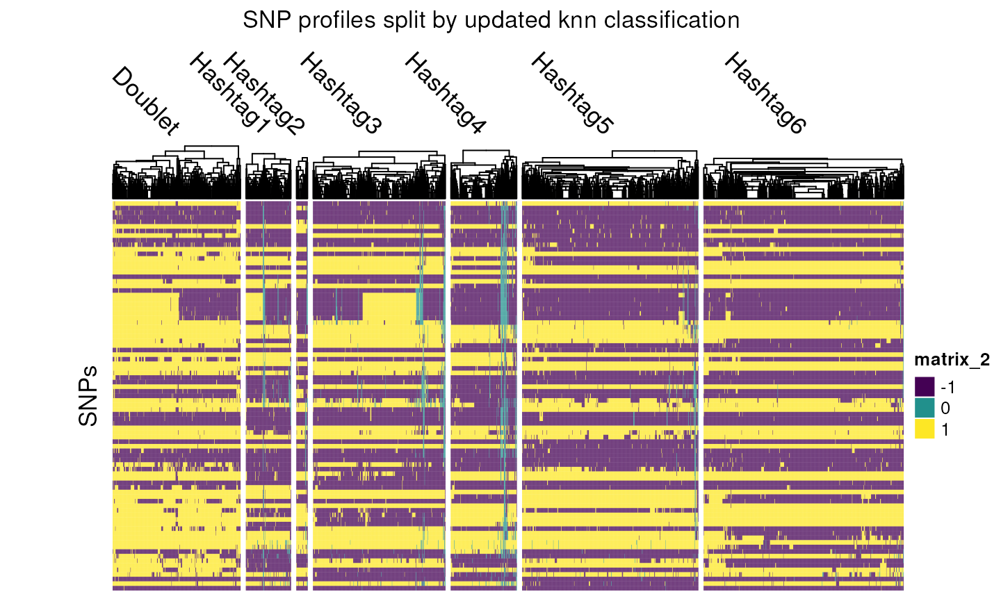
We will use our knn method to reassign cells based on their SNP profiles. The training data is the high confidence cells
set.seed(1)
multiplexed_scrnaseq_sce <- reassign(multiplexed_scrnaseq_sce,
    k = 10,
    d = 10,
    train_cells = multiplexed_scrnaseq_sce$train,
    predict_cells = multiplexed_scrnaseq_sce$predict
)

table(multiplexed_scrnaseq_sce$knn)
#>
#>  Doublet Hashtag1 Hashtag2 Hashtag3 Hashtag4 Hashtag5 Hashtag6
#>      337      119       30      349      174      464      527
hm <- Heatmap(counts(altExp(multiplexed_scrnaseq_sce, "SNP")),
    column_split = multiplexed_scrnaseq_sce$knn,
    cluster_rows = FALSE,
    show_column_names = FALSE,
    cluster_column_slices = FALSE,
    column_names_rot = 45,
    column_title_rot = -45,
    row_title = "SNPs",
    show_row_names = FALSE,
    col = colors
)

draw(hm,
    column_title = "SNP profiles split by updated knn classification",
    padding = unit(c(2, 15, 2, 2), "mm")
)
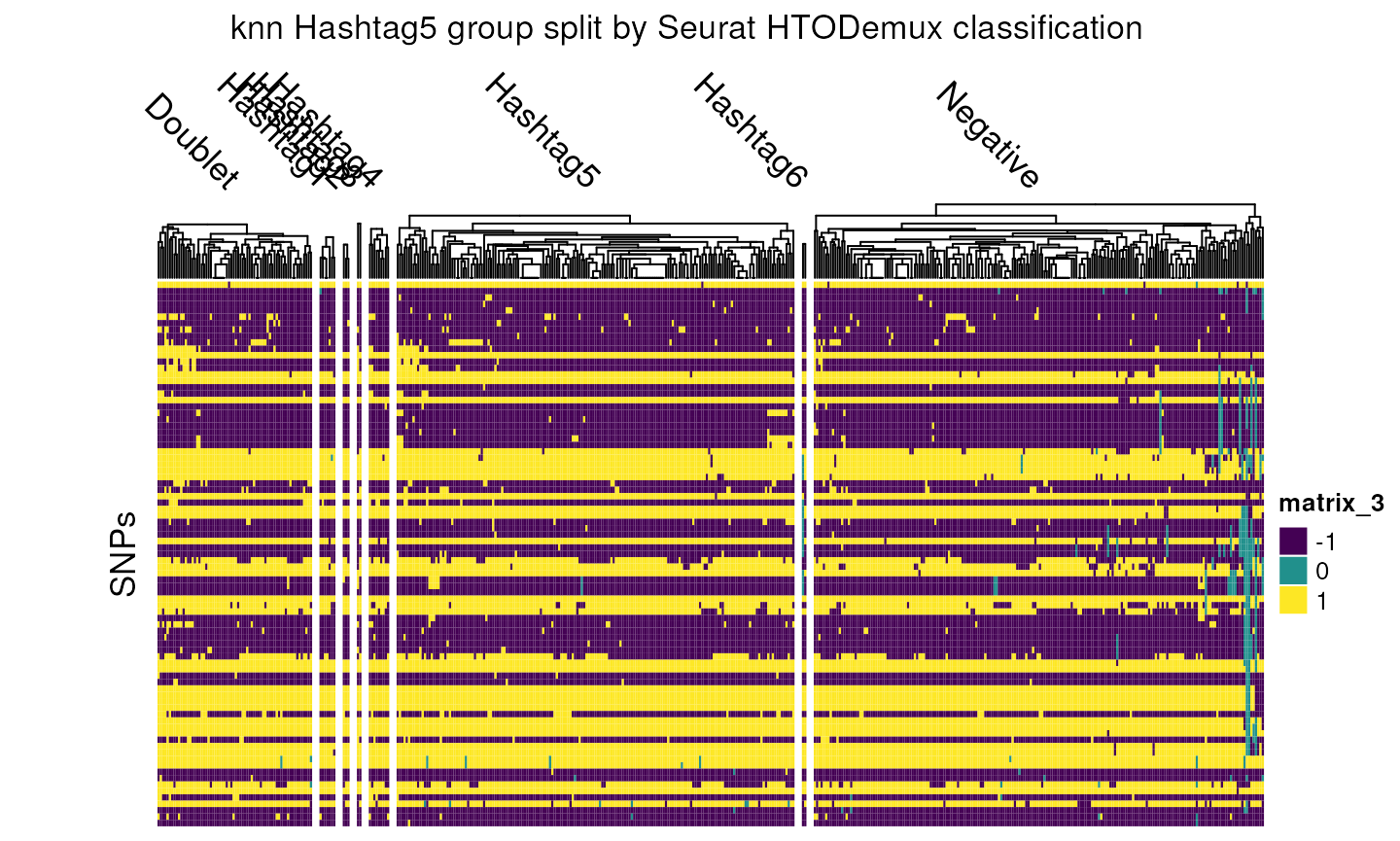
Focusing in on the knn Hashtag5 group, we see that a lot of the Negative cells have now been correctly reclassed to this group, as well as a small number of cells from other groups.
hm <- Heatmap(counts(altExp(multiplexed_scrnaseq_sce, "SNP"))[, multiplexed_scrnaseq_sce$knn == "Hashtag5"],
    column_split = multiplexed_scrnaseq_sce$seurat[multiplexed_scrnaseq_sce$knn == "Hashtag5"],
    cluster_rows = FALSE,
    show_column_names = FALSE,
    cluster_column_slices = FALSE,
    column_names_rot = 45,
    column_title_rot = -45,
    row_title = "SNPs",
    show_row_names = FALSE,
    col = colors
)

draw(hm,
    column_title = "knn Hashtag5 group split by Seurat HTODemux classification",
    padding = unit(c(2, 15, 2, 2), "mm")
)
Performance
Next we will run some basic performance checks. We subset our SingleCellExperiment object to only retain cells which we could confidently call as being from a singlet group, then split this into a training and test dataset.
sce_test <- multiplexed_scrnaseq_sce[, multiplexed_scrnaseq_sce$train == TRUE]
sce_test$knn <- NULL
sce_test$labels <- droplevels(sce_test$labels)
sce_test
#> class: SingleCellExperiment
#> dim: 259 1045
#> metadata(2): doubletClassify_between_threshold
#>   doubletClassify_between_resultsMat
#> assays(2): counts logcounts
#> rownames(259): RPL22 CDC42 ... MT-ND5 MT-CYB
#> rowData names(0):
#> colnames(1045): AAACCTGAGCGTCAAG-1 AAACCTGAGGCGTACA-1 ...
#>   ACTTTCAGTAAGAGAG-1 ACTTTCAGTAAGTTCC-1
#> colData names(14): orig.ident nCount_RNA ... predict labels
#> reducedDimNames(0):
#> mainExpName: RNA
#> altExpNames(2): HTO SNP

sce_test$train2 <- rep(FALSE, length(sce_test$train))
sce_test$train2[seq_len(500)] <- TRUE

sce_test$test <- sce_test$train2 == FALSE
Comparing the predicted labels in the test dataset with the hidden high confidence labels, we see excellent agreement.
sce_test <- reassign(sce_test, k = 3, train_cells = sce_test$train2, predict_cells = sce_test$test)

table(sce_test$labels[sce_test$test == TRUE], sce_test$knn[sce_test$test == TRUE])
#>
#>            Doublet Hashtag1 Hashtag2 Hashtag3 Hashtag4 Hashtag5 Hashtag6
#>   Hashtag1       1       35        0        0        0        0        0
#>   Hashtag2       1        0       10        0        0        0        0
#>   Hashtag3       0        0        0      122        0        0        0
#>   Hashtag4       0        0        0        0       46        0        0
#>   Hashtag5       1        0        0        0        0      193        1
#>   Hashtag6       0        0        0        0        0        0      135
We can also show that that the model can correct misclassified cells when predicted back on the training data. We create a new vector “labels2” which is initially identical to the labels used in training previously.
sce_test$knn <- NULL

sce_test$labels2 <- droplevels(sce_test$labels)

table(sce_test$labels, sce_test$labels2)
#>
#>            Hashtag1 Hashtag2 Hashtag3 Hashtag4 Hashtag5 Hashtag6
#>   Hashtag1       62        0        0        0        0        0
#>   Hashtag2        0       15        0        0        0        0
#>   Hashtag3        0        0      226        0        0        0
#>   Hashtag4        0        0        0      102        0        0
#>   Hashtag5        0        0        0        0      348        0
#>   Hashtag6        0        0        0        0        0      292
We then randomly reassign 25 cells from Hashtag5 to Hashtag2 in the training data. Predicting the model back on itself we see that in the new predicted labels, the 25 altered have been correctly reclassified back to Hashtag5
sce_test$labels2[which(sce_test$labels2 == "Hashtag5")[1:25]] <- "Hashtag2"

table(sce_test$labels, sce_test$labels2)
#>
#>            Hashtag1 Hashtag2 Hashtag3 Hashtag4 Hashtag5 Hashtag6
#>   Hashtag1       62        0        0        0        0        0
#>   Hashtag2        0       15        0        0        0        0
#>   Hashtag3        0        0      226        0        0        0
#>   Hashtag4        0        0        0      102        0        0
#>   Hashtag5        0       25        0        0      323        0
#>   Hashtag6        0        0        0        0        0      292

sce_test <- reassign(sce_test,
    train_cells = sce_test$train,
    predict_cells = sce_test$train
)

table(sce_test$labels, sce_test$knn)
#>
#>            Doublet Hashtag1 Hashtag2 Hashtag3 Hashtag4 Hashtag5 Hashtag6
#>   Hashtag1       0       62        0        0        0        0        0
#>   Hashtag2       0        0       15        0        0        0        0
#>   Hashtag3       0        0        0      226        0        0        0
#>   Hashtag4       0        0        0        0      102        0        0
#>   Hashtag5       1        0        0        0        0      346        1
#>   Hashtag6       0        0        0        0        0        0      292
For the knn Hashtag6 group, we see mostly good agreement with the original demuxmix labels. However, it appears one cell now being called a Hashtag6 was originally called Hashtag5. Again, we can investigate this by visualising the corresponding SNP profile. In doing so, we can see that this most likely is a true Hashtag6.
hm <- Heatmap(counts(altExp(sce_test, "SNP"))[, sce_test$knn == "Hashtag6"],
    column_split = sce_test$labels[sce_test$knn == "Hashtag6"],
    cluster_rows = FALSE,
    show_column_names = FALSE,
    cluster_column_slices = FALSE,
    column_names_rot = 45,
    column_title_rot = -45,
    row_title = "SNPs",
    show_row_names = FALSE,
    col = colors
)

draw(hm,
    column_title = "knn Hashtag6 group split by demuxmix classification",
    padding = unit(c(2, 15, 2, 2), "mm")
)
Session Info
sessionInfo()
#> R version 4.3.1 (2023-06-16)
#> Platform: x86_64-pc-linux-gnu (64-bit)
#> Running under: Ubuntu 22.04.2 LTS
#>
#> Matrix products: default
#> BLAS:   /usr/lib/x86_64-linux-gnu/openblas-pthread/libblas.so.3
#> LAPACK: /usr/lib/x86_64-linux-gnu/openblas-pthread/libopenblasp-r0.3.20.so;  LAPACK version 3.10.0
#>
#> locale:
#>  [1] LC_CTYPE=en_US.UTF-8       LC_NUMERIC=C
#>  [3] LC_TIME=en_US.UTF-8        LC_COLLATE=en_US.UTF-8
#>  [5] LC_MONETARY=en_US.UTF-8    LC_MESSAGES=en_US.UTF-8
#>  [7] LC_PAPER=en_US.UTF-8       LC_NAME=C
#>  [9] LC_ADDRESS=C               LC_TELEPHONE=C
#> [11] LC_MEASUREMENT=en_US.UTF-8 LC_IDENTIFICATION=C
#>
#> time zone: UTC
#> tzcode source: system (glibc)
#>
#> attached base packages:
#> [1] grid      stats4    stats     graphics  grDevices utils     datasets
#> [8] methods   base
#>
#> other attached packages:
#>  [1] CiteFuse_1.12.0             kableExtra_1.3.4
#>  [3] EnsDb.Hsapiens.v86_2.99.0   dittoSeq_1.12.0
#>  [5] ggpubr_0.6.0                ggplot2_3.4.2
#>  [7] SeuratObject_4.1.3          Seurat_4.3.0.1
#>  [9] viridisLite_0.4.2           ComplexHeatmap_2.16.0
#> [11] demuxSNP_0.99.15            ensembldb_2.24.0
#> [13] AnnotationFilter_1.24.0     GenomicFeatures_1.52.1
#> [15] AnnotationDbi_1.62.2        VariantAnnotation_1.46.0
#> [17] Rsamtools_2.16.0            Biostrings_2.68.1
#> [19] XVector_0.40.0              SingleCellExperiment_1.22.0
#> [21] SummarizedExperiment_1.30.2 Biobase_2.60.0
#> [23] GenomicRanges_1.52.0        GenomeInfoDb_1.36.1
#> [25] IRanges_2.34.1              S4Vectors_0.38.1
#> [27] BiocGenerics_0.46.0         MatrixGenerics_1.12.3
#> [29] matrixStats_1.0.0           BiocStyle_2.28.0
#>
#> loaded via a namespace (and not attached):
#>   [1] progress_1.2.2            goftest_1.2-3
#>   [3] vctrs_0.6.3               spatstat.random_3.1-5
#>   [5] digest_0.6.33             png_0.1-8
#>   [7] shape_1.4.6               ggrepel_0.9.3
#>   [9] deldir_1.0-9              parallelly_1.36.0
#>  [11] magick_2.7.4              MASS_7.3-60
#>  [13] pkgdown_2.0.7             reshape2_1.4.4
#>  [15] httpuv_1.6.11             foreach_1.5.2
#>  [17] withr_2.5.0               xfun_0.39
#>  [19] ellipsis_0.3.2            survival_3.5-5
#>  [21] memoise_2.0.1             ggsci_3.0.0
#>  [23] mixtools_2.0.0            systemfonts_1.0.4
#>  [25] ragg_1.2.5                zoo_1.8-12
#>  [27] GlobalOptions_0.1.2       pbapply_1.7-2
#>  [29] DEoptimR_1.1-0            prettyunits_1.1.1
#>  [31] KEGGREST_1.40.0           promises_1.2.0.1
#>  [33] httr_1.4.6                rstatix_0.7.2
#>  [35] restfulr_0.0.15           globals_0.16.2
#>  [37] fitdistrplus_1.1-11       rhdf5filters_1.12.1
#>  [39] demuxmix_1.2.0            rhdf5_2.44.0
#>  [41] rstudioapi_0.15.0         miniUI_0.1.1.1
#>  [43] generics_0.1.3            curl_5.0.1
#>  [45] zlibbioc_1.46.0           ScaledMatrix_1.8.1
#>  [47] ggraph_2.1.0              polyclip_1.10-4
#>  [49] randomForest_4.7-1.1      GenomeInfoDbData_1.2.10
#>  [51] xtable_1.8-4              stringr_1.5.0
#>  [53] desc_1.4.2                doParallel_1.0.17
#>  [55] evaluate_0.21             S4Arrays_1.0.5
#>  [57] BiocFileCache_2.8.0       hms_1.1.3
#>  [59] bookdown_0.34             irlba_2.3.5.1
#>  [61] colorspace_2.1-0          filelock_1.0.2
#>  [63] ROCR_1.0-11               reticulate_1.30
#>  [65] spatstat.data_3.0-1       magrittr_2.0.3
#>  [67] lmtest_0.9-40             later_1.3.1
#>  [69] viridis_0.6.4             lattice_0.21-8
#>  [71] spatstat.geom_3.2-4       future.apply_1.11.0
#>  [73] robustbase_0.99-0         scattermore_1.2
#>  [75] XML_3.99-0.14             scuttle_1.10.1
#>  [77] cowplot_1.1.1             RcppAnnoy_0.0.21
#>  [79] class_7.3-22              pillar_1.9.0
#>  [81] nlme_3.1-162              iterators_1.0.14
#>  [83] compiler_4.3.1            beachmat_2.16.0
#>  [85] stringi_1.7.12            tensor_1.5
#>  [87] GenomicAlignments_1.36.0  plyr_1.8.8
#>  [89] crayon_1.5.2              abind_1.4-5
#>  [91] BiocIO_1.10.0             locfit_1.5-9.8
#>  [93] sp_2.0-0                  graphlayouts_1.0.0
#>  [95] bit_4.0.5                 dplyr_1.1.2
#>  [97] codetools_0.2-19          textshaping_0.3.6
#>  [99] BiocSingular_1.16.0       bslib_0.5.0
#> [101] GetoptLong_1.0.5          plotly_4.10.2
#> [103] mime_0.12                 splines_4.3.1
#> [105] circlize_0.4.15           Rcpp_1.0.11
#> [107] dbplyr_2.3.3              sparseMatrixStats_1.12.2
#> [109] knitr_1.43                blob_1.2.4
#> [111] utf8_1.2.3                clue_0.3-64
#> [113] fs_1.6.3                  listenv_0.9.0
#> [115] DelayedMatrixStats_1.22.1 ggsignif_0.6.4
#> [117] tibble_3.2.1              Matrix_1.6-0
#> [119] statmod_1.5.0             svglite_2.1.1
#> [121] tweenr_2.0.2              pkgconfig_2.0.3
#> [123] pheatmap_1.0.12           tools_4.3.1
#> [125] cachem_1.0.8              RSQLite_2.3.1
#> [127] rvest_1.0.3               DBI_1.1.3
#> [129] fastmap_1.1.1             rmarkdown_2.23
#> [131] scales_1.2.1              ica_1.0-3
#> [133] broom_1.0.5               sass_0.4.7
#> [135] patchwork_1.1.2           BiocManager_1.30.21.1
#> [137] carData_3.0-5             RANN_2.6.1
#> [139] farver_2.1.1              tidygraph_1.2.3
#> [141] yaml_2.3.7                bayesm_3.1-5
#> [143] rtracklayer_1.60.0        cli_3.6.1
#> [145] purrr_1.0.1               webshot_0.5.5
#> [147] leiden_0.4.3              lifecycle_1.0.3
#> [149] dbscan_1.1-11             uwot_0.1.16
#> [151] bluster_1.10.0            kernlab_0.9-32
#> [153] backports_1.4.1           BiocParallel_1.34.2
#> [155] gtable_0.3.3              rjson_0.2.21
#> [157] ggridges_0.5.4            progressr_0.13.0
#> [159] parallel_4.3.1            limma_3.56.2
#> [161] jsonlite_1.8.7            edgeR_3.42.4
#> [163] bitops_1.0-7              bit64_4.0.5
#> [165] Rtsne_0.16                spatstat.utils_3.0-3
#> [167] BiocNeighbors_1.18.0      jquerylib_0.1.4
#> [169] highr_0.10                metapod_1.8.0
#> [171] dqrng_0.3.0               segmented_1.6-4
#> [173] lazyeval_0.2.2            shiny_1.7.4.1
#> [175] htmltools_0.5.5           sctransform_0.3.5
#> [177] rappdirs_0.3.3            glue_1.6.2
#> [179] RCurl_1.98-1.12           rprojroot_2.0.3
#> [181] scran_1.28.2              BSgenome_1.68.0
#> [183] gridExtra_2.3             igraph_1.5.0.1
#> [185] R6_2.5.1                  tidyr_1.3.0
#> [187] labeling_0.4.2            cluster_2.1.4
#> [189] Rhdf5lib_1.22.0           compositions_2.0-6
#> [191] DelayedArray_0.26.7       tidyselect_1.2.0
#> [193] ProtGenerics_1.32.0       tensorA_0.36.2
#> [195] ggforce_0.4.1             xml2_1.3.5
#> [197] car_3.1-2                 future_1.33.0
#> [199] rsvd_1.0.5                munsell_0.5.0
#> [201] KernSmooth_2.23-21        data.table_1.14.8
#> [203] htmlwidgets_1.6.2         RColorBrewer_1.1-3
#> [205] biomaRt_2.56.1            rlang_1.1.1
#> [207] spatstat.sparse_3.0-2     spatstat.explore_3.2-1
#> [209] Cairo_1.6-0               fansi_1.0.4